Winning Kaggle Competition is a Piece of Cake!
Introduction
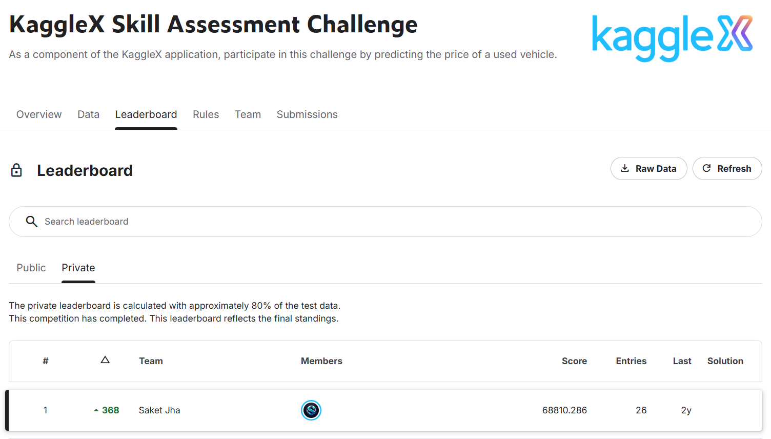
This post is about how I won the KaggleX Skill Assessment Machine Learning Competition. Disclaimer: I was just a beginner in machine learning and Kaggle competitions when I started. This competition ran for about 20 days, and I improved day by day and climbed up the leaderboard. Initially, I was ranked around 368-ish on the private leaderboard, but when the competition ended, the tables turned and I was Rank 1.
Talking about my background, I had just completed my freshman year at the National Institute of Technology Karnataka (NITK) and was on my summer break from April 15th till mid-July, so I had plenty of time. My interest in machine learning started in my first semester when I went to a flagship IEEE event at NITK called IEEE Eureka. I didn’t even know what machine learning was back then, but I was fascinated. Also, it was kind of trending at that time around 2023, ChatGPT and LLMs were on a roll and AI was everywhere so I thought, why not give it a try?
That IEEE bootcamp boosted my interest in machine learning. From there, I started learning through Andrew Ng’s course on Coursera (btw it’s one of the goated courses for ML and DL). I also watched YouTube channels like:
- StatQuest by Josh Starmer
- 3Blue1Brown for calculus and math intuition
Also, Math I and Math II in college helped a lot in understanding gradients, linear algebra, series, and calculus.
By the start of my second year, I had completed Andrew Ng’s ML course 1 and tried out models like linear regression, logistic regression, and basic data preprocessing. Then I started watching coding videos related to ML and came across Kaggle. Initially, it felt too complicated, but later I realized it’s just like LeetCode is for DSA, Kaggle is for AI and data science. A lot of Kaggle competitions are hosted by big tech companies.
I tried some starter competitions, but my performance was not that great:
- Multi-Class Prediction of Obesity Risk → 1064 / 3587 (Top ~29.66%)
- Binary Classification with a Bank Churn Dataset → 1188 / 3632 (Top ~32.71%)
- Titanic: Machine Learning from Disaster → 967 / 2938 (Top ~32.91%)
- Rohlik Orders Forecasting Challenge → 783 / 1017 (Top ~77.00%)
Then came the KaggleX Skill Assessment Machine Learning Competition, which was a 20 day long competition. I was really excited because it felt like a great opportunity to test my skills and learn from others. This competition was also an entry point for the Kaggle Cohort 2024 mentorship for building open-source stuff, so I was really hyped.
Even though my previous performance wasn’t great, I was determined to give it my best shot and learn as much as possible from the experience.
KaggleX Skill Assessment Challenge
The KaggleX Skill Assessment Challenge was part of the KaggleX Fellowship application process. Along with the application form, participants had to complete this competition to demonstrate their practical machine learning and data science skills.
The core task of the competition was simple:
- Predict the price of a used vehicle based on given features like brand, mileage, engine details, transmission, etc.
This was a regression problem, and submissions were evaluated using Root Mean Squared Error (RMSE), meaning lower scores were better.
\[RMSE = \sqrt{\frac{1}{n} \sum_{i=1}^{n} (y_i - \hat{y}_i)^2}\]Where:
- $n$ = number of samples
- $y_i$ = actual value
- $\hat{y}_i$ = predicted value
For me, it turned out to be a really good learning experience and eventually, a winning one
Here are my final scores and results from the competition:
Dataset Description
The training dataset contained:
- ~52,893 rows (after dropping missing values)
- 13 columns (features + target)
Features
The dataset included the following features:
-
id→ unique identifier -
brand→ car brand (BMW, Audi, Ford, etc.) -
model→ specific car model -
model_year→ year of manufacture -
milage→ total distance driven -
fuel_type→ type of fuel (Gasoline, Hybrid, etc.) -
engine→ engine description (contained horsepower and capacity info in text form) -
transmission→ type of transmission -
ext_col→ exterior color -
int_col→ interior color -
accident→ accident history -
clean_title→ whether the title is clean or not -
price→ target variable (car price)
Key Observation
One important thing about the dataset was:
- The
enginecolumn was not structured -
It contained mixed information like:
- Horsepower (HP)
- Engine capacity (L)
- Engine type
This became a very important feature engineering opportunity later.
Files Provided
The competition provided three main files:
- train.csv → training data with target (
price) - test.csv → test data (no
price, needed for submission) - sample_submission.csv → format for submission
Feature Engineering
In this part, I mainly focused on making the raw data more useful for the model. Some columns already looked good, but the engine column had a lot of useful information hidden inside text, so I extracted that.
Extracting Horsepower and Engine Capacity
The engine column looked something like:
"375HP 3.5L V6 Cylinder Engine""300HP 3.0L Straight 6 Cylinder"
So I extracted:
- Horsepower → from
XXXHP - Engine capacity → from
XXXL
This helped convert text into numerical features.
def get_horse_power(x, df):
    hp = []
    for i in x:
        if i.split()[0].endswith('HP'):
            hp.append(float(i.split()[0].strip('HP')))
        else:
            hp.append(np.nan)
    df['horse power'] = hp
    return df

train_df = get_horse_power(train_df['engine'], train_df)
test_df = get_horse_power(test_df['engine'], test_df)
def get_capacity(x, df):
    capacity = []
    x_new = [i.split() for i in x]

    for i in x_new:
        if len(i) >= 2 and i[1].endswith('L'):
            capacity.append(float(i[1].strip('L')))
        else:
            capacity.append(np.nan)

    df['capacity'] = capacity
    return df

train_df = get_capacity(train_df['engine'], train_df)
test_df = get_capacity(test_df['engine'], test_df)
Preprocessing Steps
After extracting features, some values were missing. I filled them using the mean.
from sklearn.impute import SimpleImputer

imputer = SimpleImputer(strategy='mean')
imputer.fit(train_inputs[numeric_cols])

train_inputs[numeric_cols] = imputer.transform(train_inputs[numeric_cols])
test_inputs[numeric_cols] = imputer.transform(test_inputs[numeric_cols])
Since models can’t directly use text, I converted categorical columns into numbers using one-hot encoding.
from sklearn.preprocessing import OneHotEncoder

encoder = OneHotEncoder(sparse=False, handle_unknown='ignore')
encoder.fit(train_inputs[categorical_cols])

encoded_cols = list(encoder.get_feature_names_out(categorical_cols))

train_inputs[encoded_cols] = encoder.transform(train_inputs[categorical_cols])
test_inputs[encoded_cols] = encoder.transform(test_inputs[categorical_cols])
For numerical columns, I also scaled values between 0 and 1.
from sklearn.preprocessing import MinMaxScaler

scaler = MinMaxScaler()
scaler.fit(train_inputs[numeric_cols])

train_inputs[numeric_cols] = scaler.transform(train_inputs[numeric_cols])
test_inputs[numeric_cols] = scaler.transform(test_inputs[numeric_cols])
What Else Could Be Done (Advanced Ideas)
I didn’t go very deep here, but some more things that could be done:
- Extract number of cylinders from engine (V6, V8, etc.)
- Convert
model_year→ car age - Combine features (like horsepower per liter)
- Frequency encoding for
brand - Use embeddings for categorical features
- Use text embeddings on
modelorengine
Feature Selection
After creating new features, I didn’t use everything directly. I selected only the features that I felt were actually useful for predicting price.
I mainly focused on:
- Keeping meaningful features
- Removing unnecessary columns
- Avoiding noise
What Features I Used
I selected the following input features:
brandmodel_yearmilagefuel_typehorse powercapacitytransmission
Target variable:
price
Code for Selecting Features
input_cols = ['brand', 'model_year', 'milage', 'fuel_type',
              'horse power', 'capacity', 'transmission']

target_col = 'price'

train_inputs = train_df[input_cols].copy()
train_targets = train_df[target_col].copy()
test_inputs = test_df[input_cols].copy()
Using Correlation & Covariance Matrix
I used a correlation matrix to understand how numerical features are related to the target (price).
Why I used this:
- To see which features are strongly related to price
- To identify useless features
- To check if some features are redundant
Code for Correlation Matrix
import seaborn as sns
import matplotlib.pyplot as plt

corr_matrix = train_df[numeric_cols + ['price']].corr()

plt.figure(figsize=(8,6))
sns.heatmap(corr_matrix, annot=True, cmap='coolwarm')
plt.title("Correlation Matrix")
plt.show()
- Some features had strong correlation with price
- Some had very low correlation → not very useful
- Helped me understand which features matter more
I also checked covariance to understand how features vary together.
Why I used this:
- To see how features change together
- To detect relationships between variables
- To get a rough idea of feature influence
Covariance is similar to correlation but not normalized. It can show the direction of the relationship (positive or negative) and the strength in terms of actual values.
cov_matrix = train_df[numeric_cols + ['price']].cov()
print(cov_matrix)
My Approach
I didn’t overcomplicate feature selection. I mainly:
- Used domain intuition (what affects car price)
- Checked correlation
- Removed obvious unnecessary features
Experimenting with Models
After preprocessing and selecting features, I started trying different machine learning models to see what works best.
I didn’t assume any model would work. I just tested multiple models and compared their performance.
I created a dictionary of models along with their parameters and tried all of them.
This helped me:
- Quickly compare models
- Avoid writing repetitive code
- See which models perform better
Models
- Linear Regression
- SGD Regressor
- Decision Tree
- Random Forest
- Gradient Boosting
- XGBoost
- LightGBM
- MLP Regressor (Neural Network)
- CatBoost
Code for Trying Multiple Models
from sklearn.base import RegressorMixin

models: dict[RegressorMixin, dict[str, float]] = {

    LinearRegression: {
        'n_jobs': -1
    },

    SGDRegressor: {
        'eta0': 0.001,
        'max_iter': 2000,
        'penalty': 'l1',
        'learning_rate': 'adaptive'
    },

    DecisionTreeRegressor: {
        'max_depth': 32,
        'max_features': 'sqrt',
        'max_leaf_nodes': 100,
        'min_samples_leaf': 4
    },

    RandomForestRegressor: {
        'n_estimators': 400,
        'max_depth': 32,
        'min_samples_split': 10,
        'min_samples_leaf': 4,
        'n_jobs': -1
    },

    GradientBoostingRegressor: {
        'learning_rate': 0.06,
        'n_estimators': 900,
    },

    XGBRegressor: {
        'n_estimators': 400,
        'max_depth': 10,
        'learning_rate': 0.01,
        'subsample': 0.5,
    },

    LGBMRegressor: {
        'n_estimators': 500,
        'num_leaves': 32,
        'learning_rate': 0.01,
        'subsample': 0.7,
    },

    MLPRegressor: {
        'activation': 'identity',
        'solver': 'adam',
        'batch_size': 32,
        'max_iter': 400,
        'random_state': 42,
        'beta_1': 0.5,
    },

    CatBoostRegressor: {
        'n_estimators': 500,
        'od_type': 'Iter',
        'bootstrap_type': 'Bernoulli',
    },
}
Instead of manually checking results, I used my evaluation pipeline:
- Trained each model
- Calculated RMSE, MAE, and R²
-
Compared validation scores
- Linear models didn’t perform well
- Decision Trees overfit easily
- Random Forest was a good baseline
- Boosting models performed the best
The best ones were:
- CatBoost
- LightGBM
- XGBoost
Why Boosting Models Worked Better
From what I saw:
- Data had non-linear relationships
- Simple models couldn’t capture patterns
- Boosting models handled it much better
Model Evaluation Strategy
After defining multiple models, I needed a proper way to evaluate and compare them. Instead of manually training each model and checking results, I created a small evaluation pipeline.
I wanted to:
- Train models easily
- Compare them fairly
- Check both train and validation performance
I wrote a function that:
- Takes a model and its parameters
- Trains it on training data
- Evaluates it on validation data
- Returns multiple metrics
Code for Evaluating a Single Model
def evaluate_model(model : type[RegressorMixin],
                   params : dict,
                   X_train : np.ndarray,
                   train_targets : np.ndarray,
                   X_val: np.ndarray,
                   val_targets :np.ndarray) -> tuple[float,float,float,float,float,float]:

    regressor = model(**params).fit(X_train, train_targets)
    train_preds = regressor.predict(X_train)
    val_preds = regressor.predict(X_val)

    train_mae = mean_absolute_error(train_targets, train_preds)
    val_mae = mean_absolute_error(val_targets, val_preds)

    train_rmse = mean_squared_error(train_targets, train_preds, squared=False)
    val_rmse = mean_squared_error(val_targets, val_preds, squared=False)

    train_r2 = r2_score(train_targets, train_preds)
    val_r2 = r2_score(val_targets, val_preds)

    return (train_mae, val_mae, train_rmse, val_rmse, train_r2, val_r2)
Trying Multiple Models Together
Then I wrote another function to test all models at once.
This helped me:
- Save time
- Compare all models in one place
- Avoid repetitive code
Code for Trying All Models
def try_models(model_dict: dict[RegressorMixin,dict[str,float]],
               X_train: np.array,
               train_targets: np.array,
               X_val: np.array,
               val_targets: np.array) -> pd.DataFrame:

    results = Parallel(n_jobs=-1)(
        delayed(evaluate_model)(model, params, X_train, train_targets, X_val, val_targets)
        for model, params in model_dict.items()
    )

    metrics = ['train_mae', 'val_mae', 'train_rmse', 'val_rmse', 'train_r2', 'val_r2']
    results_dict = {metric: [result[i] for result in results] for i, metric in enumerate(metrics)}

    df = pd.DataFrame({
        'models': list(model_dict.keys()),
        'params': list(model_dict.values()),
        **results_dict
    })

    return df
- I could quickly see which model performs better
- I focused mainly on validation RMSE
- I also checked train vs validation gap to detect overfitting
Baseline Model (CatBoost)
After trying multiple models, I saw that boosting models were performing better. So I decided to use CatBoost as my baseline model.
From the results, I picked the best parameters for CatBoost:
best_cbr_params = {
    'n_estimators': 500,
    'od_type': 'Iter',
    'bootstrap_type': 'Bernoulli',
    'verbose': 0
}
Training the Baseline Model
I trained CatBoost using these parameters and evaluated it on validation data.
- Train RMSE → ~51,454
- Validation RMSE → ~77,474
- Train R² → negative
-
Validation R² → negative
- The model was performing very poorly
- Negative R² means it was worse than predicting the mean
- High RMSE showed predictions were far off
Hyperparameter Tuning (Optuna)
After seeing that my baseline CatBoost model was performing badly, I decided to properly tune the model instead of guessing parameters.
I used Optuna for this.
I defined a search space for CatBoost and let Optuna try different combinations to minimize RMSE.
I focused on:
- Learning rate
- Number of trees
- Regularization
- Sampling parameters
Code for Optuna Tuning
import optuna

def objective(trial):

    params = {
        "n_estimators": trial.suggest_int("n_estimators", 800, 1000),
        "learning_rate": trial.suggest_float("learning_rate", 0.005, 0.006),
        "l2_leaf_reg": trial.suggest_float("l2_leaf_reg", 1, 2),
        "colsample_bylevel": trial.suggest_float("colsample_bylevel", 0.6, 0.8),
        "subsample": trial.suggest_float("subsample", 0.8, 1),
        "min_data_in_leaf": trial.suggest_int("min_data_in_leaf", 150, 200),
        "max_bin": trial.suggest_int("max_bin", 120, 180),
        "od_wait": trial.suggest_int("od_wait", 50, 80, step=10),
        "od_type": 'Iter',
        "bootstrap_type": 'Bernoulli',
        "random_seed": 42,
        "verbose": 0,
    }

    model = CatBoostRegressor(**params)
    model.fit(X_train, train_targets, eval_set=[(X_val, val_targets)])

    preds = model.predict(X_val)
    rmse = np.sqrt(mean_squared_error(val_targets, preds))

    return rmse

study = optuna.create_study(direction="minimize")
study.optimize(objective, n_trials=150)
Final Best Parameters
After running 150 trials, these were the best parameters:
-
n_estimators→ ~900+ -
learning_rate→ ~0.005–0.006 -
l2_leaf_reg→ ~1–2 -
colsample_bylevel→ ~0.6–0.8 -
subsample→ ~0.8–1 -
min_data_in_leaf→ ~150–200 -
max_bin→ ~120–180 -
od_wait→ ~50–80
Key Learnings & Takeaways
This competition taught me a lot, especially as a beginner.
What I Learned
- Start simple and improve step by step
- Feature engineering is very important
- Good preprocessing makes a big difference
- Don’t rely on just one model
- Boosting models work really well for tabular data
What Helped Me Improve
- Trying multiple models
- Proper evaluation (train vs validation)
- Using Optuna for tuning
- Learning from Kaggle discussions and notebooks
Final Takeaway
I didn’t do anything extremely complex.
I just:
- Kept experimenting
- Learned from mistakes
- Improved step by step
References
Here are some resources that helped me during the competition:
-
Kaggle Discussion Forums (very useful for ideas and approaches)
Enjoy Reading This Article?
Here are some more articles you might like to read next: